Code

# Packages
library(knitr)
library(brms)
library(ggthemes)
library(scales)
library(kableExtra)
library(posterior)
library(tidyverse)

# Options for sampling
options(
  brms.backend = "rstan",
  mc.cores = parallel::detectCores(logical = FALSE)
  )

# Function for tables
k2 <- function(x, escape = TRUE) {
  x %>% 
    kbl(digits = 2, escape = escape) %>% 
    kable_classic_2("striped", full_width = FALSE, html_font = "Arial")
}

# Plotting theme
theme_set(
  theme_few() +
  theme(
    axis.title.y = element_blank(),
    legend.title = element_blank(), 
    panel.grid.major = element_line(linetype = "dotted", linewidth = .1),
    legend.position = "bottom", 
    legend.justification = "left"
  )
)

# Download and uncompress McNeish and Hamaker materials if not yet done
path <- "materials/materials.zip"
if (!file.exists(path)) {
  dir.create("materials", showWarnings = FALSE)
  download.file(
    "https://files.osf.io/v1/resources/wuprx/providers/osfstorage/5bfc839601593f0016774697/?zip=",
    destfile = path
  )
  unzip(path, exdir = "materials")
}

Warning

I am currently studying this model implementation in more detail. It seems that there are some pieces missing, and results regarding some parameters seem unreliable. So if you want to use this in your own work, please ensure appropriate model performance with a parameter recovery simulation. Take everything below with a grain of salt. I’ll update here once I learn more about this model’s performance.

While drafting this entry, I asked for help with coding this up in brms on the Stan forums: https://discourse.mc-stan.org/t/latent-mean-centering-latent-covariate-models-in-brms/29424. I couldn’t have figured it out without the help of all those people who answered. Thanks!

The earlier drafts and mistakes I made in coding the brms model up can be found in the Git history of this file 😄

Introduction

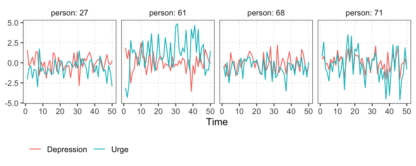
Within cluster centering, or person-mean centering (psychologists’ clusters are typically persons), is an easy but essential data processing step. For example consider the example data of 100 people’s ratings of urge to smoke and depression, collected over 50 days with one response per day (McNeish and Hamaker 2020) ¹, shown in Table 1 and Figure 1.

¹ Grab a free copy at https://osf.io/j56bm/download. I couldn’t figure if this example data is real or simulated, or what the measurement instruments were.

Code

d <- read_csv(
  "materials/Data/Two-Level Data.csv", 
  col_names = c("urge", "dep", "js", "hs", "person", "time")
) %>% 
  select(-hs, -js) %>% 
  relocate(person, time, 1)

d <- d %>% 
  # Grand mean center both variables
  mutate(across(c(urge, dep), list(c = ~ . - mean(.)))) %>% 
  group_by(person) %>% 
  mutate(
    across(
      c(urge_c, dep_c), 
      list(
        # Between-person center (= person's mean)
        b = ~ mean(.), 
        # Within-person center (= deviation from person's mean)
        w = ~ . - mean(.)
      ),
      .names = "{.col}{.fn}"
    )
  ) %>% 
  ungroup()

Table 1: Example longitudinal data (McNeish & Hamaker, 2020)
person	time	urge	dep	urge_c	dep_c	urge_cb	urge_cw	dep_cb	dep_cw
1	1	0.34	0.43	0.33	0.42	-0.31	0.64	-0.19	0.61
1	2	-0.48	-0.68	-0.49	-0.69	-0.31	-0.18	-0.19	-0.51
1	3	-4.44	-1.49	-4.45	-1.50	-0.31	-4.14	-0.19	-1.31
1	4	-4.19	-0.74	-4.20	-0.75	-0.31	-3.89	-0.19	-0.56
1	5	-0.91	-0.52	-0.92	-0.53	-0.31	-0.61	-0.19	-0.34
2	1	1.65	0.68	1.64	0.66	-0.48	2.12	-0.02	0.68
2	2	0.31	1.49	0.30	1.48	-0.48	0.78	-0.02	1.49
2	3	0.46	0.03	0.45	0.02	-0.48	0.94	-0.02	0.03
2	4	-1.09	-1.02	-1.10	-1.03	-0.48	-0.62	-0.02	-1.02
2	5	1.67	1.07	1.66	1.06	-0.48	2.14	-0.02	1.07
Note: Only displaying two participants' first five observations. _c: grand mean centered; _cb: between-person centered (ie. person mean); _cw: within-person centered.

The first four variables in Table 1 are the original data values, indicating the person and timepoint of measurement, urge to smoke, and depression. I’ve then created the grand-mean, between-person, and within-person variables by simple data transformations. Between-person centered variables are person-specific means, and within-person centered variables are deviations around that person’s mean.

Code

set.seed(999)
d %>% 
  filter(person %in% sample(1:100, 4)) %>% 
  select(1:4) %>% 
  pivot_longer(urge:dep) %>% 
  rename(Time = time) %>% 
  mutate(name = factor(name, labels = c("Depression", "Urge"))) %>% 
  ggplot(aes(Time, value, col = name)) +
  geom_line(linewidth = .5) +
  facet_wrap("person", nrow = 1, labeller = label_both)

Figure 1: Four persons’ depression and urge to smoke over time

However, the person-mean is an unknown quantity, and centering on the observed value rather than an estimate of the true “latent” quantity can be problematic. Specifically, observed mean centering leads to Nickell’s (negative bias in autoregressive effects) and Lüdtke’s (bias in other time-varying effects) biases (McNeish and Hamaker 2020, 617–18). Essentially these problems arise from not considering that the person means are unobserved, latent quantities, but instead treating them as values known without uncertainty.

So, what to do? McNeish and Hamaker (2020) and others discuss latent mean centering, which accounts for uncertainty in the person-means appropriately, and thus debiases the estimated coefficients. Latent mean centering is done inside the model, and means treating the means as estimated parameters. However, I have only been able to find examples that do this latent mean centering in MPlus, such as (McNeish and Hamaker 2020). Therefore my goal here is to reproduce their model with the free and open source software Stan front-end brms.

Single-level AR(1) model

To begin with, we replicate the authors’ basic N=1 model predicting the urge to smoke from the urge to smoke on a previous measurement occasion, and the current level of depression. Because we are modelling one person’s data only, there is no need for centering, but this model serves as a useful starting point for our quest.

Following (McNeish and Hamaker 2020), we assume that Urge at time $t$ is normally distributed around a mean $\mu_t$ with standard deviation $\sigma$. We then model the mean on an intercept, on Urge at the previous measurement occasion, and on the current level of depression²:

² I’ve used the more common $\phi$ (phi) throughout than the $\varphi$ used by M&P

\[\begin{align*} \text{Urge}_{t} &\sim N(\mu_{t}, \sigma^2), \\ \mu_{t} &= \alpha + \phi\text{Urge}_{(t-1)} + \beta\text{Dep}_{t} \end{align*} \tag{1}\]

This is straightforward. We first create a lagged urge variable, and then fit the model. Notice though that this will lead to one missing data point because the first value doesn’t have a lagged value. We confirm that our estimates are in line with those reported in the paper

Code

# Estimate model
fit_p5 <- brm(
  urge ~ urge1 + dep,
  family = gaussian(),
  data = d %>% 
    # Pick one individual (same as used in M&H2020)
    filter(person == 5) %>% 
    # Create lagged urge
    mutate(urge1 = lag(urge)),
  file = "fit_p5"
)

Code

# Show table of coefficients' posterior summaries
as_draws_df(fit_p5) %>% 
  select(1:4) %>% 
  mutate(sigma_sq = sigma^2, .keep = "unused") %>% 
  summarise_draws(median, ~quantile2(., probs = c(.025, .975))) %>% 
  mutate(
    variable = str_c(
      variable, 
      c(" ($\\alpha$)", " ($\\phi$)", " ($\\beta$)", " ($\\sigma^2$)")
    ),
    across(c(median, q2.5, q97.5), ~number(., .01)),
    `Result (brms)` = str_glue("{median} [{q2.5}, {q97.5}]"),
    Authors = c(
      "0.07 [-0.24, 0.39]", 
      "0.35 [0.25, 0.46]", 
      "2.43 [2.12, 2.75]", 
      "1.36 [0.92, 2.20]"
    )
  ) %>% 
  select(-c(median:q97.5)) %>% 
  k2(escape = FALSE) %>% 
  footnote("I've no idea how to render the math here, SRY", footnote_as_chunk = TRUE)

variable	Result (brms)	Authors
b_Intercept ($\alpha$)	0.08 [-0.25, 0.40]	0.07 [-0.24, 0.39]
b_urge1 ($\phi$)	0.35 [0.24, 0.47]	0.35 [0.25, 0.46]
b_dep ($\beta$)	2.43 [2.12, 2.76]	2.43 [2.12, 2.75]
sigma_sq ($\sigma^2$)	1.34 [0.92, 2.05]	1.36 [0.92, 2.20]
Note: I've no idea how to render the math here, SRY

Multilevel AR(1) model

Above, we modelled a single person’s urge to smoke on their previous urge to smoke and current depression. Here, we attempt to model 100 individuals’ data in a single multilevel model. Before worrying about latent mean centering, we can estimate this model using the observed mean centered values shown in Table Table 1. The authors’ model of these data is

\[\begin{align*} \text{Urge}_{ti} &\sim N(\mu_{ti}, \sigma^2), \\ \mu_{ti} &= \bar{\alpha} + \alpha_i + (\bar{\phi}+\phi_i)\text{Urge}^c_{(t-1)i} + (\bar{\beta} + \beta_i)\text{Dep}^c_{ti}, \\ (\alpha_i, \phi_i, \beta_i) &\sim MVN(\pmb{0}, \Sigma), \end{align*} \tag{2}\]

where we now have a subscript $i$ for participants, parameters with bars (population-level) and without (person-specific, with subscripts $i$), and the variance-covariance matrix for the latter, where all covariances are set to zero as in (McNeish and Hamaker 2020). Notice that the the subscripted parameters are deviations with a mean of zero, so we can talk about e.g. $\bar{\alpha} + \alpha_2$ as person 2’s intercept. $\text{Urge}^c_{(t-1)i}$ and $\text{Dep}^c_{ti}$ are the within-person centered values of urge to smoke on the previous timepoint and depression, respectively (_cw values in Table Table 1.) We can fit this model with brms with a small modification of the previous model

Code

# Create lagged variable
d <- d %>% 
  group_by(person) %>% 
  mutate(
    urge1 = lag(urge),
    urge_cw1 = lag(urge_cw)
    ) %>% 
  ungroup()

# Estimate model
fit_observed <- brm(
  urge ~ urge_cw1 + dep_cw + (urge_cw1 + dep_cw || person),
  family = gaussian(),
  data = d,
  file = "brm-fit-observed-mean-centered"
)

We now estimated the model using observed person mean centering. These estimates are very close to the ones reported in authors’ Table 4, because there are so many observations per person. (Note this is probably not the best example because of this, and also because I don’t really know what the data are from the paper). Importantly, we have not estimated the latent depression variable, so that is missing

Code

# Show table of coefficients' posterior summaries
as_draws_df(fit_observed) %>% 
  select(1:7) %>% 
  mutate(
    across(c(starts_with("sd_"), "sigma"), ~.^2)
  ) %>% 
  # mutate(sigma_sq = sigma^2, .keep = "unused") %>% 
  summarise_draws(median, ~quantile2(., probs = c(.025, .975))) %>% 
  mutate(
    variable = str_c(
      variable, 
      c(" ($\\alpha$)", " ($\\phi$)", " ($\\beta$)",
        " ($\\sigma^2_{\\alpha}$)", " ($\\sigma^2_{\\phi)}$", 
        " ($\\sigma^2_{\\beta})$", " ($\\sigma^2$)")
      ),
    across(c(median, q2.5, q97.5), ~number(., .01)),
    `Result (brms)` = str_glue("{median} [{q2.5}, {q97.5}]"),
    Authors = c(
      "-0.01 [-0.18, 0.16]",
      " 0.21 [0.17, 0.24]",
      " 0.80 [0.61, 0.95]",
      " 0.60 [0.44, 0.83]",
      " 0.02 [0.01, 0.03]",
      " 0.79 [0.61, 0.95]",
      " 1.14 [1.09, 1.19]"
    )
  ) %>% 
  select(-c(median:q97.5)) %>% 
  k2()

variable	Result (brms)	Authors
b_Intercept ($\alpha$)	0.01 [-0.16, 0.18]	-0.01 [-0.18, 0.16]
b_urge_cw1 ($\phi$)	0.20 [0.16, 0.23]	0.21 [0.17, 0.24]
b_dep_cw ($\beta$)	0.78 [0.63, 0.96]	0.80 [0.61, 0.95]
sd_person__Intercept ($\sigma^2_{\alpha}$)	0.68 [0.52, 0.91]	0.60 [0.44, 0.83]
sd_person__urge_cw1 ($\sigma^2_{\phi)}$	0.02 [0.01, 0.03]	0.02 [0.01, 0.03]
sd_person__dep_cw ($\sigma^2_{\beta})$	0.77 [0.57, 1.01]	0.79 [0.61, 0.95]
sigma ($\sigma^2$)	1.14 [1.10, 1.19]	1.14 [1.09, 1.19]

The problem then boils down to figuring out how to get the quantities $\text{Urge}^c_{(t-1)i}$ and $\text{Dep}^c_{ti}$. Usually, we calculate them from data as deviations from the person’s observed mean, like we did above in Table 1. However, here’ we want to use latent-mean centering:

\[\begin{align*} \text{Urge}^n_{(t-1)i} &= \text{Urge}^c_{(t-1)i} + \text{Urge}^b_i, \\ \text{Dep}^n_{ti} &= \text{Dep}^c_{ti} + \text{Dep}^b_i \end{align*} \tag{3}\]

brms

It turns out that specifying this model with latent mean centering is fairly straightforward with brms. First, we will need to specify a non-linear formula where we name all parameters, and then another one that specifies that one of the predictors is a parameter too. Thanks to Mauricio Garnier-Villarreal, Ethan McCormick, Simon Brauer, Joran Jongerling, and others who helped out with my Stan discourse question to figure out the syntax!

Here goes. We specify a formula of urge on the named parameters and predictors, as you do with brms’ nonlinear formulas. Then in the subsequent lines, each parameter is specified their own model. The trick is to predict the latent means inside another nlf(), and then the predictor there in another model formula. That’s it! And because this is a nonlinear formula, we need to assign some priors.

Code

latent_formula <- bf(
  urge ~ alpha + phi*(urge1 - alpha) + beta*(dep - depb),
  alpha ~ 1 + (1 | person),
  phi ~ 1 + (1 | person),
  beta ~ 1 + (1 | person),
  nlf(depb ~ depCB),
  depCB ~ 1 + (1 | person),
  nl = TRUE
) +
  gaussian()

p <- get_prior(latent_formula, data = d) %>%
  mutate(
    prior = case_when(
      class == "b" & coef == "Intercept" ~ "normal(0, 1)",
      class == "sd" & coef == "Intercept" ~ "student_t(7, 0, 1)",
      TRUE ~ prior
    )
  )

fit_latent <- brm(
  latent_formula,
  data = d,
  prior = p,
  control = list(adapt_delta = 0.99),
  file = "brm-fit-latent-mean-centered"
)

We can then compare our parameters’ posteriors to those in McNeish and Hamaker:

Code

as_draws_df(fit_latent) %>% 
  select(1:9) %>% 
  mutate(
    across(c(starts_with("sd_"), "sigma"), ~.^2)
  ) %>% 
  summarise_draws(median, ~quantile2(., probs = c(.025, .975))) %>% 
  mutate(variable = str_replace(variable, "sd_person__", "var_")) %>% 
  mutate(
    variable = str_c(
      variable, 
      c(" ($\\alpha$)", " ($\\phi$)", " ($\\beta$)", " (DepB)",
        " ($\\sigma^2_{\\alpha}$)", " ($\\sigma^2_{\\phi)}$", 
        " ($\\sigma^2_{\\beta})$", " ($\\sigma^2_{DepB})$",
        " ($\\sigma^2$)")
      ),
    across(c(median, q2.5, q97.5), ~number(., .01)),
    `Result (brms)` = str_glue("{median} [{q2.5}, {q97.5}]"),
    Authors = c(
      "-0.01 [-0.18, 0.16]",
      " 0.21 [0.17, 0.24]",
      " 0.80 [0.61, 0.95]",
      " 0.01 [-0.02, 0.04]",
      " 0.60 [0.44, 0.83]",
      " 0.02 [0.01, 0.03]",
      " 0.79 [0.61, 0.95]",
      " 0.01 [0.00, 0.01]",
      " 1.14 [1.09, 1.19]"
    )
  ) %>% 
  select(-c(median:q97.5)) %>% 
  k2(escape = FALSE)

variable	Result (brms)	Authors
b_alpha_Intercept ($\alpha$)	-0.12 [-0.32, 0.08]	-0.01 [-0.18, 0.16]
b_phi_Intercept ($\phi$)	0.21 [0.18, 0.25]	0.21 [0.17, 0.24]
b_beta_Intercept ($\beta$)	0.78 [0.61, 0.94]	0.80 [0.61, 0.95]
b_depCB_Intercept (DepB)	-0.10 [-0.23, 0.03]	0.01 [-0.02, 0.04]
var_alpha_Intercept ($\sigma^2_{\alpha}$)	0.56 [0.41, 0.78]	0.60 [0.44, 0.83]
var_phi_Intercept ($\sigma^2_{\phi)}$	0.02 [0.01, 0.03]	0.02 [0.01, 0.03]
var_beta_Intercept ($\sigma^2_{\beta})$	0.76 [0.58, 1.03]	0.79 [0.61, 0.95]
var_depCB_Intercept ($\sigma^2_{DepB})$	0.01 [0.00, 0.05]	0.01 [0.00, 0.01]
sigma ($\sigma^2$)	1.14 [1.10, 1.19]	1.14 [1.09, 1.19]

Looking carefully, there is some small difference in the intercepts of urge and mean depression. Their variances, however, are identical to M&H. I think this might have something to do with how MPlus / brms works and how the priors are specified, so I am not worried about that. Or maybe with how the lagged variable is treated.

Conclusion

Because it is this easy to specify latent means in brms, I think I will be using them much more often from now on, especially if my sample size per person is small. I don’t think this will make much of a difference after that sample size is greater than, say, the magic number 30.

Let me know if you have any comments!

References

Enders, Craig K., and Davood Tofighi. 2007. “Centering Predictor Variables in Cross-Sectional Multilevel Models: A New Look at an Old Issue.” Psychological Methods 12 (2): 121–38. https://doi.org/10.1037/1082-989X.12.2.121.

McNeish, Daniel, and Ellen L. Hamaker. 2020. “A Primer on Two-Level Dynamic Structural Equation Models for Intensive Longitudinal Data in Mplus.” Psychological Methods 25 (5): 610–35. https://doi.org/10.1037/met0000250.

Reuse

https://creativecommons.org/licenses/by/4.0/

Citation

BibTeX citation:

@online{vuorre2023,
  author = {Vuorre, Matti},
  title = {Latent Mean Centering with Brms},
  date = {2023-01-01},
  url = {https://vuorre.netlify.app/posts/latent-mean-centering},
  langid = {en}
}

For attribution, please cite this work as:

Vuorre, Matti. 2023. “Latent Mean Centering with Brms.” January 1, 2023. https://vuorre.netlify.app/posts/latent-mean-centering.

Latent mean centering with brms

Introduction

Single-level AR(1) model

Multilevel AR(1) model

brms

Conclusion

See also

References

Reuse

Citation